A Simple Guide to Automatically Coloring Cells in Excel

Hey there, let me show you an awesome trick that’ll make your Excel spreadsheets look amazing! In this guide, I’ll walk you through how to automatically color code cells in Excel.

First things first, you may be wondering why you would want to color code cells in the first place. Well, let me tell you, it makes your data much easier to read and understand. Instead of just staring at a bunch of plain numbers or text, color coding helps you quickly identify different categories or values.

Now, let’s get started. Here’s what you need to do:

Step 1: Open your Excel spreadsheet and select the cells you want to color code. You can choose a whole column, a specific range, or just a few cells – it’s up to you!

Step 2: Once you’ve selected the cells, go to the “Home” tab in the Excel ribbon. Look for the “Conditional Formatting” button and click on it. A dropdown menu will appear.

Step 3: In the dropdown menu, you’ll see various options for applying conditional formatting. For color coding, we’ll choose “Highlight Cells Rules” and then “Equal To…”

Step 4: A dialog box will pop up, allowing you to set the formatting rule. This is where the real magic happens! In the box next to “Equal To”, type in the value or text that you want to color code.

Step 5: Now, let’s choose a color for your highlighted cells. Click on the “Format…” button in the dialog box, and another dialog box will appear. Here, you can select a color from the palette or customize your own.

Step 6: Once you’ve chosen your color, click “OK” to close the dialog boxes. You’ll be taken back to the main Excel window, where you’ll see your cells magically color coded!

And that’s it! With just a few simple steps, you’ve learned how to automatically color code cells in Excel. It’s a fantastic way to make your data more visually appealing and easier to understand. Plus, it adds a touch of professionalism to your spreadsheets.

So, go ahead and give it a try. Play around with different colors and formatting options to find the perfect look for your data. I guarantee you’ll impress your colleagues, friends, or whoever you’re sharing your spreadsheet with. Happy Excel-ing!

Let me tell you about some useful options that can make your color coding task easier. It’s important to understand how each option works, so you can choose the best one for your job.

Highlight Duplicates

Highlighting duplicates is a basic color coding task that you can do in Excel. What it does is mark all the duplicate names in the same color. This can help you get rid of duplicate names or analyze your spreadsheet more effectively. Let me show you how to highlight duplicates.

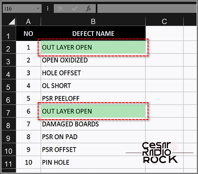
1. First, you gotta pick the cells you wanna check for duplicates. Easy, just press Ctrl + A and you’ll select all the cells in your table.
   
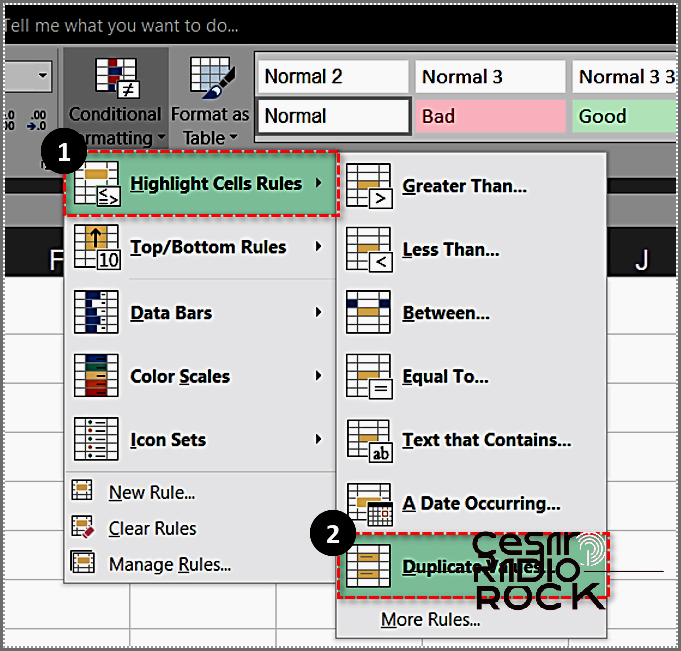
2. Now, go to the Home tab and find Conditional Formatting. It’s gonna be your best buddy for this task.
   
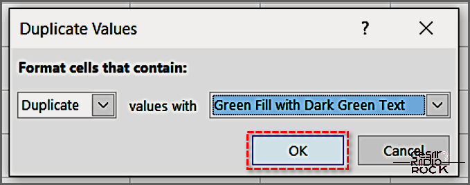
3. Click on Conditional Formatting and then on Highlight Cell Rules. Find Duplicate Values and click on it. This is where the magic happens.
   
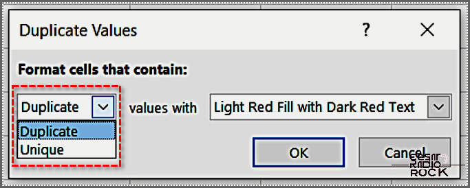
4. A fancy window will pop up, giving you options to choose from. It’s like a candy store, but for formatting cells. Cool, right?
5. So, the first thing you gotta do is pick which cells you want to color. You can go for Duplicate ones or the Unique ones. Your call!
   
6. Then, you get to choose the color. Yay for customization! Check out the available options and have fun playing with colors.
   
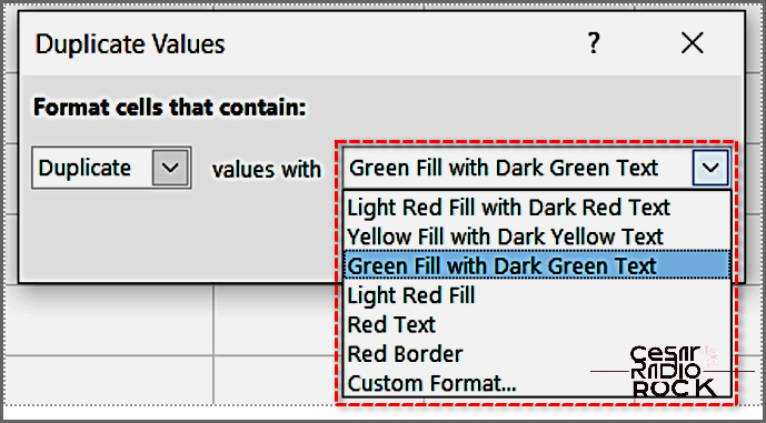
7. Hit the OK button and watch the magic unfold. Your selected cells will be highlighted according to your choices. Ta-da!
   

Sort by Color

If highlighting duplicates wasn’t enough for you, the sort by color option will blow your mind. Now you can group and sort those duplicates together, which is super helpful for big lists. Here’s how to do it:

1. Select the range of data you want to work with.
2. Go to Data -> Sort & Filter -> Sort. Get ready for the next level!
3. Pick the column you want to sort. This is where the magic happens. Prepare to be amazed!
4. Choose Cell Color for the Sort on option. Color is the key here.
5. Select a color for the Order. You’re the boss, choose whatever you want!
6. For the final touch, select On Top in the drop-down list. It’s like the cherry on top of the cake.
7. Hit OK and watch the magic happen. Your data will be sorted based on the color you picked. Amazing, right?

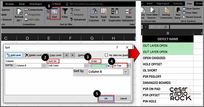
Hey there! I’ve got a neat trick for you that will make sorting your list a breeze. Not only that, but it will also bring all those pesky duplicates right to the top, so you can deal with them easily.

Highlight the Cream of the Crop

Whether we’re talking about things like geography, finances, or temperatures, the top 10 items on a list can reveal a lot about the whole list. And guess what? You can apply the same trick to highlight the bottom 10, top 10%, bottom 10%, above average, below average, and many other groups of data. Sounds cool, doesn’t it?

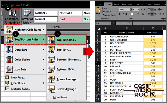
1. First things first, select the range of data you want to work with.
2. Now head over to the Home tab.
3. Click on the Conditional Formatting option.
4. Jump to the Top/Bottom Rules section.
5. Choose the Top 10 Items option.
6. A window will pop up, allowing you to adjust the number of options you want (you can go beyond 10 or have less than 10 if you wish).
7. Next, pick a fill color that will make your highlighted items stand out.
8. Lastly, hit the OK button.

Advanced Features

Alright, let’s take a look at some more powerful options available in Excel. But don’t fret, they’re just as straightforward as the previous ones.

Visualize Differences with Data Bars

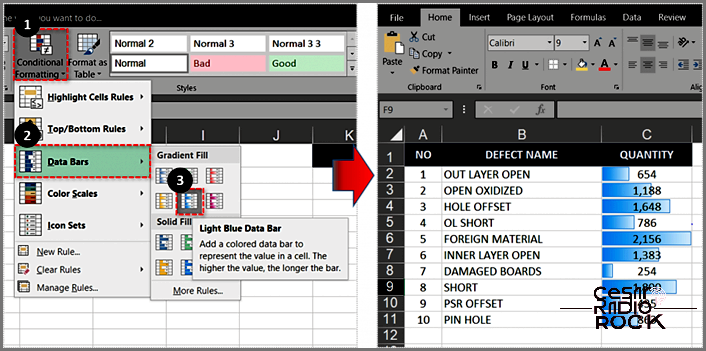
Data bars do something pretty cool – they display a bar within each cell, and the length of the bar represents the value in relation to other cells. Check out this image for a better idea:

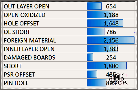
So, let me walk you through the process of choosing the specific column or range that you want to format. It’s actually pretty straightforward!

1. First, you need to select the data range that you want to format. Simply click and drag your cursor over the cells that you want to include. Easy-peasy!
2. Next, head on over to the Home tab. Yup, it’s that big ol’ tab at the top of your screen. Give it a click!
3. Now, within the Home tab, you’ll find the Conditional Formatting option. Go ahead and navigate to that. You can often find it in the toolbar or ribbon menu.
4. Once you’ve found Conditional Formatting, look for the Data Bars option. It should be nestled somewhere in there. Click on it!
5. Finally, it’s time to pick your desired color and fill style. Take a moment to explore the different options and choose the one that suits your fancy. You’ll see a preview of how it will look right there, so you can make sure it’s just right.

Hey, you did it! You’ve successfully selected the column or range that you want to format. Wasn’t too hard, was it? Now go ahead and make those spreadsheets shine with style!

Bring Your Data to Life with Icon Sets

In this tutorial, we’ll explore a powerful technique for visually representing positive, neutral, and negative values in your data. By utilizing icon sets, you can effortlessly highlight the significance of each item, making it ideal for analyzing sales and revenue breakdowns.

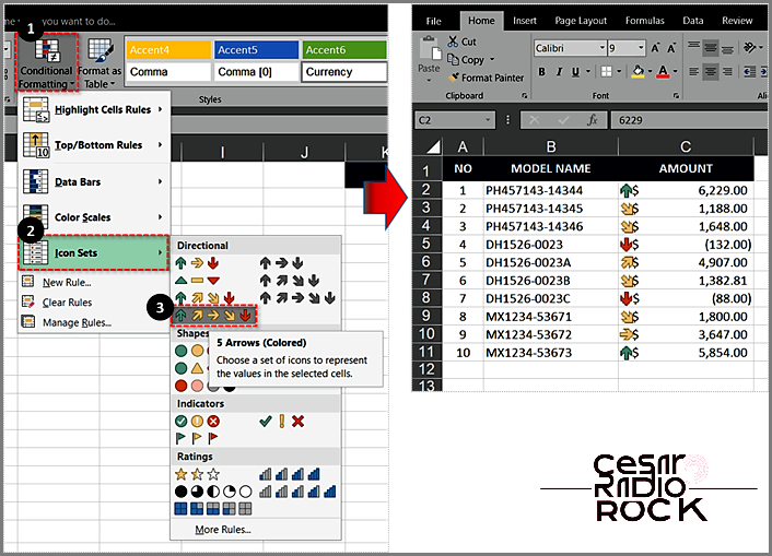
How to Format Data Using Icon Sets:

1. To format the column or range you want, select it.
2. Next, go to the Home tab.
3. From there, go to Conditional Formatting and choose Icon Sets.
4. Pick the style of icons you want to use.
5. Excel will automatically understand your data.
6. If you want to make changes, go to Conditional Formatting and click on Manage Rules.
7. Find the rule for Icon Sets and select Edit Rule.
8. You can now adjust the rules to fit your preferences.

Show Variances with Color Scales

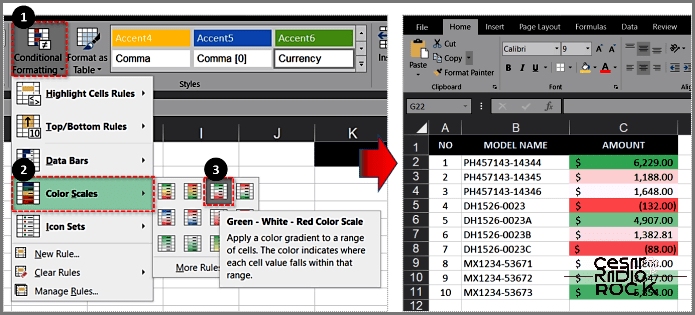
If you prefer to use Color Scales in Conditional Formatting, the process is similar to Icon Sets but with more gradients in the result.

1. Select the range you want to format.
2. In Conditional Formatting, choose Color Scales.
3. Pick the color scale you prefer.

A Seamless and Effortless Experience

Conditional formatting may seem simple, but it packs a punch when it comes to customizing your data. This handy feature really brings out the full potential of Excel – it’s not just about making your tables look good, it’s about harnessing the true power of this incredible spreadsheet program.

I’m curious to know, what unique tricks do you have up your sleeve when it comes to Excel? We all have our own methods and strategies while working with spreadsheets. So go ahead and share your wisdom in the comment section below. Feel free to give advice, ask questions, or share any tips you may have!