How to Keep the Top Row in Google Sheets Always Visible
When dealing with large spreadsheets or comparing data, it can be really helpful to freeze a row or column. This way, you can keep important headers or other information visible while scrolling through your sheet. It’s also useful to freeze the first column containing data that helps identify the rest of the cells. Learning how to freeze the top row in Google Sheets, or any column for that matter, will make your analysis a breeze.
Personally, I switch between Google Sheets and Excel depending on my clients’ preferences. Some of them like the openness and accessibility of Sheets, while others prefer the enhanced security and features of Excel. Although I have a slight bias towards Excel, both programs are pretty similar at their core.
The methods for freezing rows and columns in Google Sheets vary slightly depending on whether you’re using a web browser or a mobile device. In this example, I’ll show you how to do it in the browser version of Sheets. If you’re using a mobile device, you can find most of these options in the context menu.
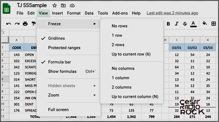
How to Freeze the Top Row in Google Sheets
Freezing rows in Google Sheets is a handy feature when you need to compare data, especially since the top row usually contains column headers. By keeping this row in place while scrolling through a large spreadsheet, you can easily make sense of the information. Here’s how you can do it:
First, open your Google Sheet in your browser.
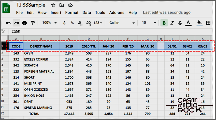
Next, select the row that you want to freeze. You can do this by clicking on the row or cell.
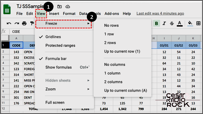
Then, go to the “View” menu and click on “Freeze.”
Finally, choose the “1 row” option.
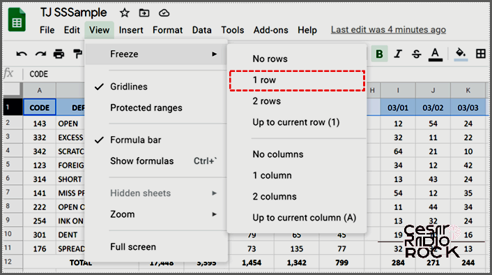
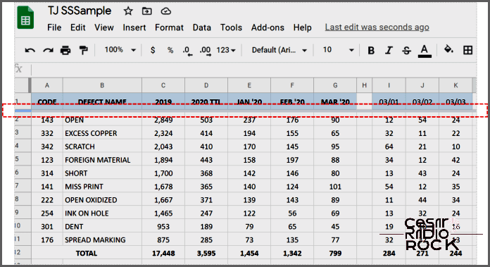
Once you have completed these steps, you will see a gray line appear underneath the row you froze. When you scroll down the sheet, the frozen row will stay in place while the rest of the sheet scrolls as usual.
If you are using a mobile device, simply tap the screen to select the row and then tap again to bring up the context menu. From there, you can choose the desired options. The same method applies for freezing multiple rows or columns, as well as unfreezing rows or columns when needed.
How to Freeze Multiple Rows in Google Sheets
If your data requires freezing more than a single row, you can freeze multiple rows in Google Sheets. This is particularly useful when you need to compare specific rows within a sheet. Here’s how:
Start by selecting the row below the last row you want to freeze.
Then, go to the “View” menu and click on “Freeze.”
Finally, choose the “Up to current row” option.
For example, let’s say you want to freeze the top three rows. Simply select row 3, go to the “View” menu, click on “Freeze,” and choose “Up to current row (3).” This will freeze the desired rows. Please note that sequential rows can be frozen, but you cannot select and freeze non-sequential rows within the same sheet.
How to Freeze a Column in Google Sheets
Columns can also contain comparative data, so it’s helpful to freeze them too. This is especially important in larger spreadsheets where category data is in column 1 or 2, and you have to scroll across to access it. Here’s how you can freeze a column in place.
- Select the column you want to freeze.
- Click on the View tab and then select Freeze.
- Choose the option to freeze 1 column.
If you click on the column header, the entire column will be highlighted. Then, just like when you froze a row, click on View and Freeze.
How to Freeze Multiple Columns in Google Sheets
The process for freezing multiple columns in Google Sheets is similar. The only difference is that instead of selecting rows, you select entire columns by clicking on their header letter or name.
- Select the columns you want to freeze.
- Click on the View tab and then select Freeze.
- Select the option to freeze up to the current column.
For example, if you want to freeze the first two columns, select them and then click on View and Freeze. You should see the option ‘Up to current column (2)’.
How to Freeze Columns and Rows in Google Sheets
You can also freeze columns and rows in Google Sheets to easily compare data across the entire spreadsheet. Simply follow the instructions for freezing a row, and then repeat the instructions for freezing a column. Gray lines will appear beside and underneath each frozen row and column, and you’re done. I won’t repeat the instructions here, just follow the steps for freezing a row and then freezing a column as mentioned above.
How to Unfreeze Rows or Columns in Google Sheets
When you click on View and Freeze, you’ll notice the option to freeze “No rows” or “No columns”. This is how you unfreeze a row or column. The wording may not be the most elegant, but the end result is the same.
- Select the columns you want to unfreeze.
- Click on the View tab and then select “No rows” or “No columns”.
The gray lines that indicate a frozen row or column will disappear, allowing you to scroll through the spreadsheet again.
