How to Hide Excel Errors with the IF and ISERROR Functions

Let’s talk about a pretty nifty trick I’ve got up my sleeve for you today. It’s all about hiding those pesky errors that can pop up in your Excel spreadsheets. You know the ones I’m talking about – those little red flags that can mess up your whole data analysis. But fear not, my friend, because I’m here to show you how to handle them like a pro.

First things first, we’re going to need two handy functions: IF and ISERROR. These bad boys are your secret weapon against errors. Here’s how they work:

The IF function is pretty straightforward. It helps us make decisions based on certain conditions. You give it a condition to evaluate, and it gives you a result based on that condition. Simple, right?

Now let’s bring in our second hero, the ISERROR function. This one’s like your trusty sidekick. It checks if a cell contains an error and gives you a TRUE or FALSE result. Think of it as the detector of all things error-related.

So here’s the big reveal: we’re going to use these two functions together to tackle those errors head-on. It’s like a dynamic duo, ready to save the day!

Here’s how it goes down:

1. We start by writing an IF formula that checks if a cell contains an error using the ISERROR function.

2. If the cell does contain an error, the IF formula will return a TRUE value. That’s our cue to take action.

3. In case of an error, we can use the IF formula to display a custom message or leave the cell empty. How fancy is that?

Here’s an example to put it all into perspective:

Let’s say we have a formula in cell A1 that’s dividing a number in cell B1 by a number in cell C1. Now, if cell C1 contains a zero (which would result in an error), we don’t want to show that error. Instead, we want to display a message like “Divide by zero error.”

To make this happen, we can use the IF and ISERROR functions together. Our formula would look something like this:

=IF(ISERROR(B1/C1), “Divide by zero error”, B1/C1)

And that’s it! With a little help from the IF and ISERROR functions, we can wave goodbye to those pesky Excel errors. Now you can impress your friends with error-free spreadsheets and be the Excel guru you were meant to be. Go forth and conquer, my friend!

Microsoft Excel is an amazing tool for tracking and managing all sorts of things, from business budgets to personal fitness. One of the great features of Excel is its ability to update formulas automatically as you enter new data. However, sometimes these formulas can produce errors when they don’t have all the necessary information. These errors, such as #DIV/0!, #VALUE!, #REF!, and #NAME?, can make your table look messy and hard to understand. Luckily, there’s a way to hide these errors using the IF and ISERROR functions. Let me show you how.

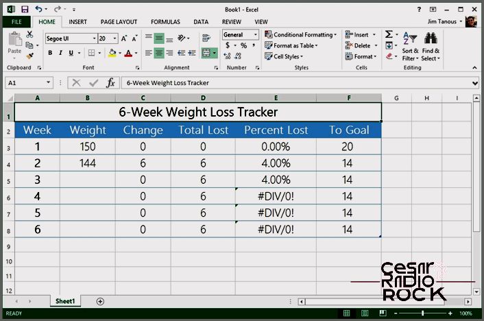
Let’s say we have a small weight loss tracking spreadsheet as an example. The problem is that the “Percent Lost” column shows a #DIV/0! error when there’s no weight entered for a particular week. We have three ways to solve this:

1. We can remove the formula for weeks with no weight and manually add it back each week. This works for small spreadsheets but not for larger ones.

2. We can use a different formula that doesn’t divide by zero. This depends on the spreadsheet and data set.

3. We can use the ISERROR function with an IF statement to define an alternate result if there’s an error. This is what I’ll show you today.

The ISERROR function tests a cell or formula and returns “true” if there’s an error, and “false” if there isn’t. You can use it by putting the formula or cell in parentheses after the function, like this: ISERROR((B5-B4)/C5). If the calculation returns an error, ISERROR will return “true”. We can then use this with the IF function.

The IF function has three parts: the test, the result if true, and the result if false. For example, IF(B5>100,0,B5) means that if the value in B5 is greater than 100, it will show 0. Otherwise, it will show the actual value of B5.

Now, let’s combine IF and ISERROR. In our weight loss spreadsheet, the formula in cell E6 produces a #DIV/0! error because it’s dividing by the previous week’s weight, which isn’t available yet. But with IF and ISERROR, we can tell Excel to ignore the error and show 0% or complete the calculation if there’s no error. Here’s the formula: IF(ISERROR(D6/B5),0,(D6/D5)).

With this formula, any errors will be replaced with zeros. As you enter new data, the affected cells will update automatically. You can use any value or formula in the IF statement, not just zeros. For example, IF(ISERROR(D6/B5),””,(D6/D5)) will show a blank space instead of a zero if there’s an error.

Just remember that IF statements can be complex, so be careful with parentheses and commas. Excel can help by color-coding formulas as you enter them.