Connecting Data to a Different Tab in Google Sheets: A Simple Guide

Hello there! Today, I’m going to show you how to link data from one tab to another in Google Sheets. It may sound a bit complicated, but don’t worry – I’ll break it down for you into easy, understandable steps. So let’s get started!

First, let me explain why you might want to do this. Imagine you have a lot of data in one tab, and you want to use some of that data in another tab without having to manually copy and paste it. Linking the data between tabs can save you time and effort. Pretty neat, right?

Here’s how you do it:

Step 1: Open up your Google Sheets document and look at the tabs at the bottom. Each tab represents a different sheet in your document.

Step 2: Click on the tab where you have the data you want to link from. For example, let’s say you have a tab called “Sales Data” and you want to link some of that data to a tab called “Summary.”

Step 3: In the “Sales Data” tab, select the cell or range of cells you want to link. You can do this by clicking and dragging your mouse over the desired cells.

Step 4: Once you have selected the cells, go up to the formula bar, which is located above the grid of cells. You should see the cell reference for the selected cells in the formula bar.

Step 5: Copy the cell reference by either right-clicking and selecting “Copy” or pressing “Ctrl+C” on your keyboard.

Step 6: Now, go to the tab where you want to link the data to – in our example, that’s the “Summary” tab.

Step 7: Select the cell where you want the linked data to appear. Again, you can do this by clicking on the desired cell.

Step 8: In the formula bar, type an equal sign (=) and then paste the cell reference you copied earlier. So, it should look something like “=Sales Data!A1” (with “Sales Data” being the name of the tab and “A1” being the cell reference).

Step 9: Press Enter on your keyboard, and voila! You should now see the data from the “Sales Data” tab linked to the “Summary” tab.

See? It’s not as complicated as it may seem. By following these steps, you can easily link data from one tab to another in Google Sheets. This little trick can save you a lot of time and help you organize your data more efficiently.

I hope you found this guide helpful. Now you can go ahead and impress your friends with your newfound Google Sheets skills! Good luck, and happy linking!

With all its cool add-ons, snazzy templates, and smooth integration with Microsoft Excel, Google Sheets has become a must-have tool for students, professionals, and even folks who just want to tidy up their music collection. It might not have Excel’s full power, but it’s a nifty free option for those who dig Google.

Maybe you’ve been rockin’ and rollin’ with Google Sheets for a while now and are ready to level up from being a Data Dabbler to becoming a Google Sheets Master. Well, guess what? The pros have got two kick-ass tricks up their sleeves that will elevate your spreadsheets to the next dimension. And the best part? They’re both simple and straightforward.

The first trick involves linking data to another tab, while the second involves pulling in data from another sheet or workbook. Pretty handy in lots of situations, trust me.

So, I’m gonna guide you through both tricks step by step, and before you know it, you’ll be a pro too.

Linking to Another Tab in Google Sheets

First things first, let’s talk about how to link to another tab in Google Sheets.

It’s as easy as pie to link a cell to another tab:

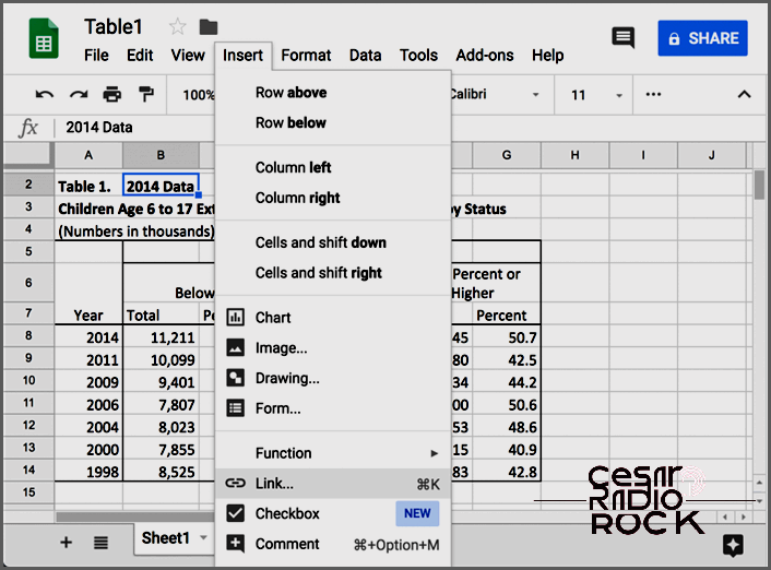
Start by selecting a cell in your sheet. It can be an empty cell or one that already has some data. Go to the ‘Insert’ menu and choose ‘Link.’ Check out the screenshot below, where I’m selecting the top cell with the text “2014 Data.”

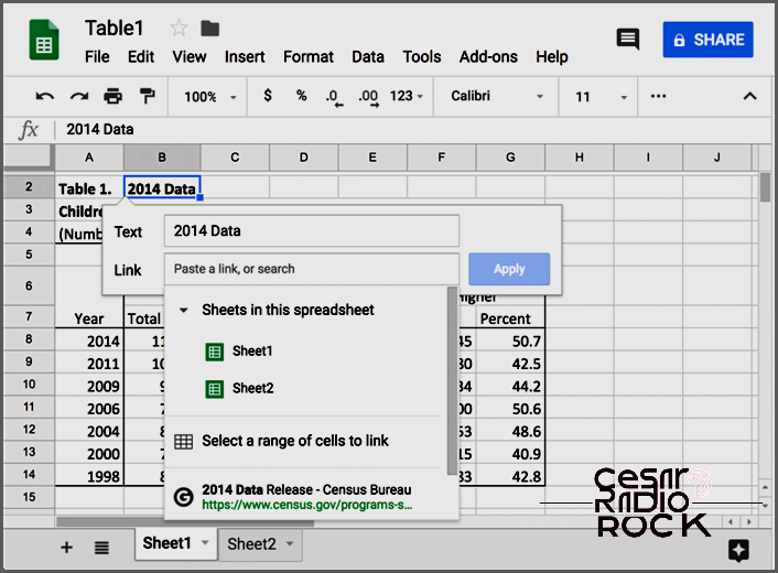
When you click on something, a dialog box will pop up on your screen. It will give you a few choices and ask you a question. It might ask if you want to connect to “Sheets in this spreadsheet” which is another tab, or if you want to select a range of cells to connect. Google, being Google, might also try to guess other sources that you could link to.

Look at the picture below. You’ll see at the very bottom, Google is asking if I want to link to census.gov because it noticed that’s where I got this data from. This feature can be really handy when you want to keep track of where you got your information.

But for now, let’s start by just linking to “Sheet2” because we’re already on “Sheet1”.

When you select a cell, something interesting happens – it turns into a hyperlink. And guess what? When you click on that cell, a pop-up shows up with a URL. Click on the URL and it will magically take you to “Sheet2” or whichever sheet you picked!

But wait, there’s more! Let’s try the other option: selecting a range of cells. When you do this, another dialog box pops up and asks, “What data?”. And here’s a pro tip: if you want, you can simply click and drag that dialog box to move it out of your way.

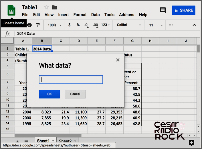
Alright, so here’s the deal – you have two options to link cells together. You can either type in the specific range of cells you want, or you can do it the easy way and just click and drag a bunch of cells. Take a look at the picture below to see an example of what I mean. In this case, I’ve chosen all the data in row 8.

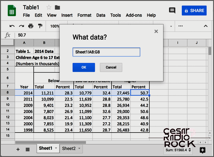
So, whenever you click on a specific cell, a link will appear. And when you click that link, all the data in row 8 will be selected. This can be really helpful if you find yourself constantly needing to select a certain set of data in your spreadsheet.

Linking to Another Workbook in Google Sheets

But what if you need to link to another workbook instead of just another tab?

Linking to a workbook in Google Sheets is a more advanced technique. It’s almost like the opposite of inserting a link to another tab or range of cells. Instead of creating a link that takes you somewhere else, you’re creating a link that pulls in data from somewhere else. It does involve some manual coding, but don’t worry, it’s actually quite simple.

To link to another workbook, you’ll need to use the IMPORTRANGE function. When you use this function, you’re telling Google Sheets to go find some data somewhere else and bring it in.

If you want, you can activate this function by going to the Insert menu, then selecting Function/Google/IMPORTRANGE. This will insert the beginning of the code you need automatically. But it’s probably easier to just do it manually. Start with an equals sign—this tells Google Sheets that you’re entering a function, not just data. Then type IMPORTRANGE.

Next, you need to tell Google Sheets where to find the data. This is done in two parts: the worksheet and the specific cell or range of cells. Each part is enclosed in quotation marks, and the whole thing is placed in parentheses. For example, if I want to import data from a cell on Sheet2 to a cell on Sheet1, I would do this:

=IMPORTRANGE(“https://docs.google.com/spreadsheets/d/1PXYv00mWphBzvknmEY2JwcPqabdFgRA6nhZfaRjFA7w/edit#gid=261974994”, “sheet2!G21”)

You can see that we have an equals sign followed by IMPORTRANGE, then the URL and the cell number, all in quotation marks and enclosed in parentheses. I’ve color-coded each part to make it easier to understand. This is how it will look in your browser:

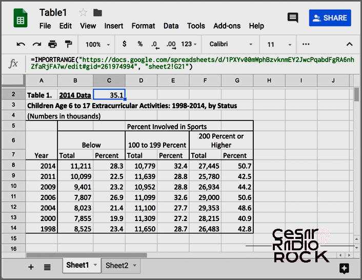
When you start using the function, you might notice a red exclamation point in the cell. If you click on the cell, you’ll see an error message telling you that the worksheets need to be linked. A pop-up button will appear, asking if you want to link them. Once you allow the sheets to be linked, you’re good to go. The cell will then retrieve the data from the other sheet.

Alternatively, you can select a range of cells by separating them with a colon, like this: “sheet2!G10:G21”. This instructs Google Sheets to grab all the data from the G column within rows 10 and 21. Just make sure that the cell you’re importing the data into has enough space. In my example, there is already data below my selected cell, C2. Therefore, Google Sheets wouldn’t allow me to import that range.

Discover More Ways to Use Google Sheets

Google Sheets is a powerful and intuitive program that allows you to create detailed spreadsheets. The best part? It’s completely free! However, it can be challenging to unlock its maximum potential on your own.

Thankfully, here at TechJunkie, we have a wide range of articles that can help you make the most of Google Sheets. These include tutorials on how to calculate time, subtract with formulas, and enable dark mode. Check them out to enhance your Google Sheets skills!

Do you have any other techniques for linking Google Sheets or workbooks? Share them with us in the comments below!